In defense of a quantitative approach to financial markets

I have the feeling that there is some subtle yet spread misconception about data-driven research in financial markets and I will take this article: Seeking Alpha – Not Even Wrong: Why Data-Mined Market Predictions Are Worse Than Useless by Justice Litle (also appearing in his website: Mercenary Trader) as a starting point for the discussion.

The article itself is born as a rant against this article on Yahoo Finance: Why Boring Is Bullish, which “infers” a 89% chance of bullish action on the S&P based on a sample of 18 previous cases where we had similar “low vol” as now.
Now, let me clearly say that the Yahoo article is indefensible for a number of reasons in my opinion (to mention a few: way too small sample size, no robustness analysis, no mention of numbers of trials that were run), so in this I agree with Mr Litle.

However Mr Litle goes beyond this and explains why equity markets cannot be “boring” right now:

“The potential trajectory of equity markets is DIRECTLY IMPACTED BY the trajectory of debt and currency markets (which are the OPPOSITE of boring now). […] “Calm before the storm boring,” maybe. Plain old boring boring? Ah, no.” […]

and eventually moves his critics to data mining in financial markets in general:

“Markets are far from simple. In fact they are very complex. As such, predictions based on data mining of a single historical variable or single cherry-picked pattern observation are almost always worse than useless because they ignore a core confluence of factors.” […]

“When it comes to predicting future outputs of complex systems, virtually ALL forms of single-variable statistical thinking are flawed.” […]

“The only way to avoid getting fooled by spurious data or superficial thinking is to put real elbow grease into truly understanding what drives markets and why…and once you have that understanding you don’t need to cherry pick or data mine because you have something better: The ability to assess a confluence of key factors in the present, as impacting important market relationships here and now.”

Now, while I agree that financial markets are very complex and that it’s very easy to be fooled, I believe that these statements about data mining are a tad too generic.
Using a single historical variable or taking into consideration the influence of multiple factors says absolutely nothing per se on how good a prediction is (and with “prediction” I refer to any kind of statistical inference over the future).

In general, to be able to make a prediction with some value one has to identify certain features (variables) that combined in a certain way have some predictive power over future events. This is true for any field and for any prediction method, be it AI or human reasoning.

The hard part of course is finding these features and combining them.

Looking at things this way, the author of the Yahoo article is just claiming that (a certain definition of) low-level of volatility has some explanatory power over future returns. What Mr Litle is responding is that monetary policy, debt and currency markets instead are better features to use, based on his experience and view of the world.

Is this really that different from properly done data mining?

The big question is whether “understanding” the causes of certain market dynamics is a key factor in making them forecastable to a certain degree (note the quotes in “understanding”).

I don’t believe this to be the case.

To make a parallel with the world of Physics, physicists certainly don’t always understand WHY certain things follow a certain law. Rather they observe a certain behaviour and they try to describe it. If along the way they can find some sort of explanation for it, the better. But there will always be an additional “why” which requires an answer (why apples fall towards the ground? -> gravity -> why gravity exist? -> relativity -> etc).

Of course a key difference with Physics is that financial markets cannot be entirely described by equations, being the results of complex interactions of billions of people. From a practical point of view this means that with a data-driven approach we have to put much more attention in developing a framework to evaluate the actual predictive power of any model, which also will hardly work “forever”.

But similar difficulties apply to any kind of discretionary trading. The very same fact that there are so many factors in play (and hence so much noise) makes it hard for our brain to analyze the situation objectively, and surely the many cognitive biases that affect us don’t help.
So our “understanding” of the causes of market movements can’t really go that far. E.g. we might understand that a certain inefficiency exists because of some institutions operating under some constraints, but we won’t know how long these constraints will stay in place or when some competitors will pick on this inefficiency reducing our profit margin or even causing the markets to behave in a totally unpredictable way.

With this I don’t want to say that using some discretion is pointless – rather I’m just trying to argue that there is a place for both in trading and I see no dualism here. Pure (properly done) data-driven research and pure macro/discretionary research lead to two different sets of opportunities that can also overlap in some situations.

Probably discretionary trading can be more responsive to changing market dynamics, whereas a data-driven approach might have his strength in the portability of the operations to different markets and in how quantifiable it is.
And in any case I strongly believe that any data-driven analysis is only as good as the thought we put into it, and likewise any type of discretionary trading can only benefit from making use of some quantitative analysis.

To comment on a last point brought up by Mr Litle:

“Yet we spend roughly zero time on data mining, with no interest in statements like “Over the past X years, the S&P did this X percent of the time.”

Why this contrast? Because markets are a complex sea of swirling and interlocking variables – and it is the historical drivers and qualitative cause-effect relationships are what have lasting value. It is not the output of a spreadsheet that matters – the pattern-based cherry picking lacking insight as to what created the results – but the qualitative relationships truly attributable to joint causation of various outcomes, on a case-by-case basis, with a very big nod to history and context.”

I agree that what matters is indeed finding some “relationships” that have real predictive power over the future. But how one finds these relationships is a complex matter and one has to  dig in the specifics of each case to find out if the analysis has some value, because generally speaking the output of a spreadsheet can be as good or as bad as any qualitative relationships one may think to hold.

Andrea

Order matching algorithms

In today’s markets dominated by High-Frequency algos, room for profits for non-HF (and more importantly, non-HF aware) guys is generally speaking reduced. The proportional performance impact of HF is likely to be bigger the smaller is your average trade and the shorter your holding period.

However, in my experience this doesn’t have to be necessary the case: simply put, as in any business you have to adapt to the competitors  and in this case one way of doing it is to pay more attention and improve the execution side of your trading. This is not always easily doable (see the “Timestamp fraud” reported by Zerohedge), but there are some low-hanging fruits that can be picked as a first step.

If this statement may sound kind of vague to you, I have an example based on my experience that supports it and that I think that could be useful to others (while hopefully not having too much of an impact on my strategies).

While all my models are fully automated, I still like to look at markets and particularly at order books when my orders are being executed.
Something that I noticed quite some time ago when trading 30y US bond futures was that whenever my limit orders were executed, I was immediately at a loss.
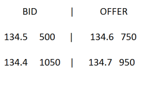
What this means is better explained by an example. Say that we had an order book that looked like this:

and that my sell limit order was included in those 750 @ 134.6.

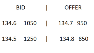
Whenever I was executed, the mid-price would then immediately move against me, and the book would then look something like this:

Basically what was happening was that my order was always one of the last to be executed, so the simple fact that it got filled meant that there were no more offers (bids) at my level, and the best bid and offer would move up (down) one tick.

A quick investigation on the CME website revealed that the cause for this was the type of order matching algo being used by the exchange, a First In, First Out (FIFO) algo.

What is a matching algorithm?
CME explains it as:

A matching algorithm is a technique to allocate matched quantities, used when an aggressor order matches with one or multiple resting orders. Algorithms apply to both outright and implied matching.

In Rajeev Ranjan’s website you can find a more in-depth introduction to Order Matching Algorithms (as well as other resources on HFT/algo trading).

In the example above, my trading model was instructed to send the limit order only when the price was close enough to my desired level, which always made me one of the last to join the queue and hence one of the last to be filled, according to the FIFO paradigm.

In practical terms, what this meant was that I was always executed in the worst possible scenarios, that is when the price would continue in the opposite direction of my order, and at the same time I was never executed in the best scenarios, that is when the price would “touch” my level and then reverse back in my favour.

As you can imagine, a simple workaround for me was to send my limit orders (when operating under FIFO matching algos) as early as possible, but generally speaking, this observation can suggest different things to different people. For day traders that are not trading in an automated fashion, operating under FIFO matching algorithms could often mean increasing one’s Maximum Adverse Execution by one tick (which can be quite a lot, depending on what one is doing ), unless one is able to play around it.

Similarly to this case, there are other situations when the order matching algo in use and trades execution in general can become as important as the strategies/trade ideas themselves.

Another example of making good use of order matching algorithms could be that of a trader operating under a pro-rata matching algorithm, typical of Eurodollar (IR) futures. If you really want a fill of X lots, you could just send an order that is somewhat bigger than X – with the extra amount being dictated by how aggressive you want/need to be – and once filled try to cancel the remaining lots (DISCLAIMER: of course by doing this you are actively risking of being filled in all the lots, so just don’t take my word on this being a good practice and do it at your own risk).

Of course paying attention to the matching algorithm is just scratching the surface of the High-Frequency world, but I would think that in some situations it’s an easy “scratch” to do and one that could directly add some value.

To conclude this post, let me clearly say that for how good our market simulator is, trades execution can’t always be modelled beforehand. This doesn’t mean that we should give up trying to make simulations as realistic (and somewhat conservative) as possible, e.g. in terms of fills and slippage (here’s a nice post on what is slippage by Prof. Tucker Balch). Rather, we should just remember that there is no real substitute for personal first hand observation and interaction with the world.
All in all, it shouldn’t really come as a surprise that simple observation is a powerful tool, being it the first step of the scientific method.

Andrea

 

Feature selection in trading algorithms

Lately I have been looking for a more systematic way to get around overfitting and in my quest I found it useful to borrow some techniques from the Machine Learning field.

If you think about it, a trading algorithm is just a form of AI applied to prices series. This statement, although possibly obvious, puts us in the position to apply a number of Machine Learning techniques to our trading strategies design.

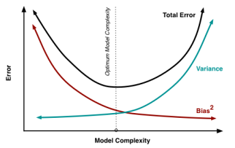
Expanding what discussed here (and here), it seems intuitive that the more features in a model, the more generally speaking the model might be subject to overfitting. This problem is known as the bias-variance trade-off and is usually summarised by the graph on the right.

As complexity increases, performance in the training set increases while prediction power degrades

What’s possibly less intuitive is that the specific features used in relation with the dynamics to predict play a key role in determining whether we are overfitting past data, so that the error behaviour showed in the graph is just a generalization.

Something particularly interesting is that the use of the very same feature (e.g. in our application an indicator, a take profit or stop loss mechanism, etc) might or might not cause overfitting according to the dynamics we are trying to fit.

The reason behind this is that some phenomena (or some times even variants of the same phenomenon) simply can’t be described by some features.

As an example, imagine you are trying to forecast the future sales of a sportwear store in Australia. A “good” feature to use could be the season of the year, as (say) Aussies are particularly keen in water sports and so springs and summers tend to show the best sales for the year.
Now imagine trying to forecast the future sales of a similar sportwear store located somewhere in the US. It might be the case that US citizens don’t have a preference for any particular season, as in the summer they practice water sports and in the winter they go skiing. In this new scenario, a model using the season of the year as a feature is more likely to result in an overfitted model because of the different underlying dynamics.

Back to financial markets, an example of this could be how a stop loss mechanism tends to be (generally speaking and according to my experience) a good feature for trend-following strategies, but not for mean-reversion strategies (and viceversa for target profit orders). A possible explanation of this could be that trends are well described by the absence of big adverse movements, but their full extension can’t be known beforehand (but this is just me trying to rationalize my empirical findings).

So, how do you understand which features are good candidates?
Luckily for us, there are a whole bunch of techniques developed in the Machine Learning field to operate feature selection. I recommend the following 2003 paper for an overview of the methods: An Introduction to variable and feature selection by Isabelle Guyon. Any text of Machine Learning should also cover some of the techniques, as it does the exceptional Stanford’s Machine Learning class in Coursera 
Any other readers’ recommendation (or comment) is of course very welcome.

Andrea

Trimmed performance estimators

This is a quick follow-up on my previous post on Quantile normalization.

Instead of removing just the top X quantile of returns/trades when optimizing a strategy’s parameters space, my recent approach has been to remove the top and bottom X quantiles, so effectively using a robust trimmed estimator of performance instead of the estimator itself.

The advantages are symmetric to those discussed in the previous post, as long as your backtest allows for realistic modelling of trades execution – e.g. if  you are using stop orders and trade bars (as opposed to tick data), you probably want to add an amount of slippage in some way proportional to the size of bar (specification needed because a conservative modelling of limit orders is easier to achieve).

Trimming out the worst returns is particular useful in case of strategies having single big losses (such are mean-reversion strategies of some kind usually), whereas trimming the best returns is more useful for strategies with big positive days (e.g. trend-following strategies).

Two (of many) possible variants are:

-To preserve autocorrelations of a strategy’s returns, one could decide to remove blocks of trades/days, instead of individual trades/days (in a similar fashion to what one does when bootstrapping blocks of trades/days).

-To preserve the number of samples in our results instead of removing the top (worst) days, one could replace them with the average/median positive (losing) days.

Something else to note is that if your performance measure makes use of std deviation (as it’s the case for Sharpe Ratio), trimming the tails of the returns from its computation is likely to result in an overestimation of the performance.

Finally, here’s the Matlab code:

———————————
normalise_excess_pnl = 1;
normalisation_quantile = 0.98;

if normalise_excess_pnl

best_daily_pnl = quantile(pnl_daily,normalisation_quantile);
worst_daily_pnl = quantile(pnl_daily,1-normalisation_quantile);

pnl_daily(pnl_daily>=best_daily_pnl ) = [];
pnl_daily(pnl_daily<=worst_daily_pnl ) = [];

end

———————————

(I usually have the variable normalise_excess_pnl automatically initialised to 1 or 0 from the external environment, according to whether or not I’m running an optimisation).

Andrea